

Computer Vision Pipeline: Key Takeaways
- A production-grade computer vision inspection pipeline has six layers: image acquisition, preprocessing, model architecture, edge inference, production system integration, and model lifecycle management.
- Most CV inspection projects fail at layers 1 and 5 (optics and integration), not at layer 3 (the model). Teams over-invest in model architecture and under-invest in lighting design and PLC/MES connectivity.
- Edge inference is non-negotiable for manufacturing. If your conveyor runs at 1 meter per second, you have roughly 200ms to capture, process, and act. Cloud round-trips consume that budget before inference begins.
- Model lifecycle management separates proof-of-concept systems from production systems. Without drift detection, retraining workflows, and version control, a CV model degrades within months of deployment.
What is a Computer Vision Inspection Pipeline?
A computer vision inspection pipeline is the end-to-end system architecture that takes a raw camera image from a manufacturing production line and converts it into an actionable quality decision (pass, fail, or rework) within milliseconds. It is not a single model or a single camera. It is six interconnected engineering layers, each with its own constraints, trade-offs, and failure modes. Getting any one layer wrong can make the entire system unreliable, regardless of how sophisticated the other layers are.
Why Does Architecture Matter More Than Model Accuracy?
Most conversations about computer vision for manufacturing start with the model. What architecture should we use? How many training images do we need? What accuracy can we expect?
These are the wrong first questions. The right first question is: what does the physical environment look like?
A model trained on perfectly lit, high-resolution images of your product will achieve 99% accuracy in the lab. Put that same model on your factory floor, where overhead fluorescents cast uneven shadows, where oil mist from CNC machines creates a haze, where conveyor vibration introduces motion blur, and accuracy drops to 80%. The model did not get worse. The images got worse.
This is why architecture, not model selection, determines whether a CV inspection system works in production. The six layers below represent the full engineering scope of what you are actually building. If you are still evaluating whether to build this in-house or buy off the shelf, we cover that build-vs-buy decision framework for CV quality inspection in a companion article.
The Six-Layer CV Inspection Pipeline
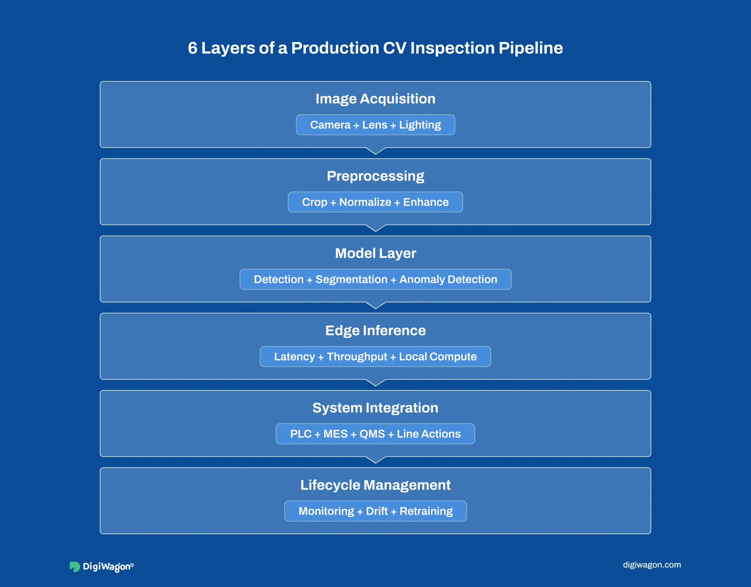
Layer 1: Image Acquisition
This is where most projects underestimate complexity. Camera selection depends on three interlocking variables:
Resolution vs. throughput. A 20MP camera captures fine surface detail but generates 60MB per frame. At 10 frames per second, that is 600MB/s of raw data. Your image pipeline needs to handle that bandwidth without dropping frames.
Lighting geometry. Backlighting reveals silhouette defects (chips, cracks). Angled lighting reveals surface topography (scratches, dents). Diffuse dome lighting eliminates shadows on curved surfaces. Most installations need multiple lighting configurations, sometimes switching between them per inspection cycle.
Lens selection. Telecentric lenses eliminate perspective distortion for dimensional measurement. Standard machine vision lenses work for surface defect detection but introduce parallax errors at the edges of the field of view.
The correct answer is almost always: work with an imaging specialist to design the optical setup before writing a single line of code. The best model in the world will not compensate for bad image acquisition. Budget 15–20% of your total project cost here.
Layer 2: Image Preprocessing
Raw camera images need processing before they reach the model. This layer handles:
- Geometric correction (undistortion, perspective transform to normalise product orientation)
- Exposure normalisation (compensating for lighting variation across shifts and seasons)
- Region-of-interest extraction (cropping to the product boundary, ignoring conveyor belt and fixtures)
- Training-time augmentation (rotation, flip, brightness jitter) to make the model tolerant of production variation
Preprocessing is often treated as trivial. It is not. A 5% improvement in image normalisation consistency can produce the same accuracy gain as doubling your training dataset.
Layer 3: Model Architecture
For defect detection in manufacturing, three model families dominate in 2026:
| Model Family | Best For | Speed | Annotation Need |
|---|---|---|---|
| YOLOv8/v9 | Detecting and localizing discrete defects (cracks, inclusions, missing components) | 30+ FPS on Jetson Orin | Bounding boxes around defects |
| U-Net / Mask R-CNN | Pixel-level segmentation for quantifying defect area, shape, and location | 10–15 FPS on Jetson Orin | Pixel-level masks per defect |
| PatchCore / EfficientAD | Anomaly detection when defect examples are scarce (new product launches) | 20+ FPS on Jetson Orin | Good-product images only (no defect labels needed) |
The choice depends on your defect taxonomy and your annotation budget. YOLO is the default for most discrete-defect problems. Anomaly detection is the right starting point when you lack historical defect data. Segmentation models are reserved for cases where defect quantification (exact area, shape metrics) is required for downstream quality reporting.
Do not default to the most complex model. A well-trained YOLOv8 model will outperform a poorly trained Mask R-CNN on the same dataset every time.
Layer 4: Edge Inference
Production CV systems run inference at the edge, not in the cloud. The math makes this non-negotiable: if your conveyor runs at 1 meter per second and your inspection field of view is 200mm, you have 200ms to capture, preprocess, infer, and act. A cloud round-trip consumes 50–200ms in network latency alone, before inference begins.
The typical edge hardware stack in 2026:
- Inference GPU: NVIDIA Jetson AGX Orin (for complex models) or Jetson Orin Nano (for simpler models)
- Cameras: GigE Vision industrial cameras with hardware triggering
- Inference runtime: NVIDIA TensorRT (for NVIDIA GPUs) or Intel OpenVINO (for Intel hardware)
- Host: Industrial PC running Ubuntu Linux, fanless, rated for factory floor temperatures
Model optimisation for edge is not optional. You will need to quantise your model from FP32 to FP16 (minimal accuracy loss) or INT8 (some accuracy loss, significant speed gain). Plan for this from day one. A model that runs at 5 FPS in FP32 can hit 30+ FPS in INT8 with TensorRT, often with less than 1% accuracy degradation.
Layer 5: Integration and Action
This is where custom systems create value that off-the-shelf platforms cannot match. A CV system that produces alerts nobody sees delivers limited value. Real value comes from integration:
PLC integration. The CV system sends pass/fail signals to the Programmable Logic Controller via Modbus TCP, PROFINET, or OPC UA. On a fail signal, the PLC stops the line or activates a diverter to route the defective product to a rework station. Latency from inference to PLC action must be under 50ms.
MES integration. Inspection results feed into the Manufacturing Execution System for real-time SPC charts, Cp/Cpk calculations, and trend analysis. Operators see quality metrics on their HMI dashboards alongside production data.
QMS integration. Defect images, classifications, and lot traceability data flow into the Quality Management System for audit trails, CAPA documentation, and customer quality reports.
Feedback loops. Inspection data triggers upstream process adjustments. If the CV system detects increasing scratch frequency, it alerts maintenance that a tooling surface needs reconditioning before the defect rate exceeds the control limit.
Layer 6: Model Lifecycle Management
A production CV model is not a deploy-and-forget system. Without lifecycle management, model accuracy degrades within months as production conditions drift.
Continuous data collection. Every inspected image (pass and fail) enters the training dataset, with operator-verified labels for model refinement.
Drift detection. Monitor model confidence scores over time. When average confidence drops below a threshold, it signals environmental change (new supplier material, seasonal lighting shift, tool wear) and triggers retraining.
A/B deployment. Run the new model in shadow mode alongside the production model, comparing classifications before swapping. Never deploy a retrained model directly to production without shadow validation.
Version control. Track which model version inspected which production lot. This is mandatory for regulatory traceability in medical device (ISO 13485) and automotive (IATF 16949) manufacturing.
Key Takeaway: Budget and timeline should reflect where CV projects actually fail. Allocate 30% of effort to optical design (Layer 1), 25% to integration (Layer 5), 20% to model training (Layer 3), 15% to lifecycle management (Layer 6), and 10% to preprocessing and edge optimisation (Layers 2 and 4).
Lessons from Building CV Pipelines: Mining Intelligence

In our work building the Mining Intelligence platform for automated visual data extraction from geological samples, we encountered the same six-layer engineering challenge. The specifics differed (geological core samples instead of manufactured parts, mineral classification instead of defect detection), but the architecture was structurally identical: image ingestion, preprocessing, model inference, and integration with downstream decision systems.
Three lessons that transferred directly:
First, we spent more engineering time on image capture standardisation than on model architecture. Getting lighting right across different sample types eliminated 40–50% of accuracy problems that we would have otherwise tried to solve with model complexity.
Second, annotation quality mattered more than annotation volume. Cleaning up 5,000 mislabeled training images produced a bigger accuracy gain than adding 15,000 new images with inconsistent labels.
Third, TensorRT quantisation (FP16 and INT8) reduced our inference time by 3–4x with less than 1% accuracy loss. Edge optimisation is not a nice-to-have. It is table stakes for any CV system that needs to run in a production environment with real-time latency constraints.
How DigiWagon Can Help
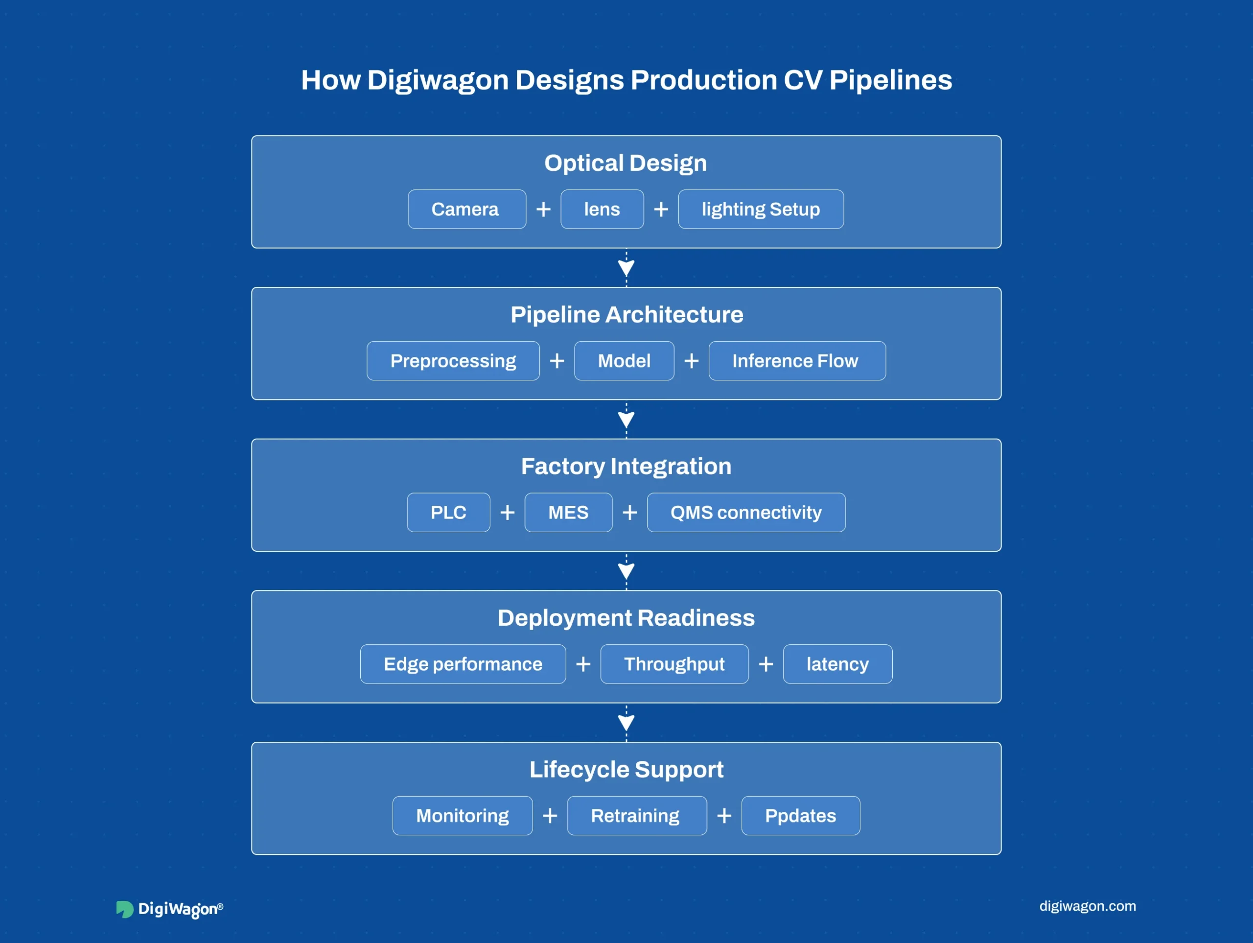
DigiWagon helps manufacturing teams design computer vision inspection systems as production-ready pipelines, not isolated model experiments.
That includes:
- Optical design for camera, lens, and lighting setup
- Pipeline architecture across preprocessing, detection, and inference
- Factory integration with PLC, MES, or QMS systems
- Edge deployment for real-time performance on the line
- Lifecycle support through monitoring, retraining, and model updates
The focus is not just model accuracy. It is building an inspection pipeline that performs reliably on the factory floor.
Build a Production-Ready CV Pipeline
Plan the full inspection system, not just the model
Related reading:
- Computer Vision for Quality Inspection: Build vs. Buy for Manufacturing CTOs – the companion decision-framework blog
- Computer Vision in Manufacturing: 5 Use Cases Driving Operational Efficiency in Germany & UAE
- Multimodal Decision Intelligence: Converging Vision, Voice, and Sensor Data in Industry 4.0
- Vertical AI: Why Generic LLMs Fail in Custom Software